In this tutorial we will learn how to solve PDEs using the Finite Element method by using Gridap.jl.

Gridap.jl is a multi-purpose FE library writen in pure Julia language. The Gridap.jl library is a very complete that supports linear and nonlinear PDE systems for scalar and vector fields, single and multi-field problems, conforming and nonconforming FE discretizations, on structured and unstructured meshes of simplices and n-cubes. One of the main advantages of Gridap.jl is that it has a very expressive API allowing one to solve complex PDEs with very few lines of code, as we will see in what follows.

Before starting the tutorial we load Gridap.

using Gridap

Problem setting

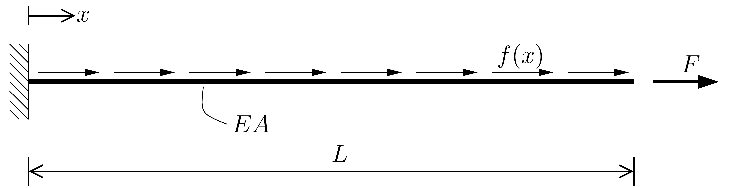
Here we consider the simple 1-dimensional rod equation. From the strong form we can derive the weak form of the problem:

Domain discretization

The first step that we need to do is to define the discretization of our domain. Since the geometry is defined by a line, we can use the CartesianDiscreteModel function. This function creates a discrete model with a Cartesian grid for arbitrary topological dimensions, i.e. a line in 1D, a square in 2D, a cube in 3D, ... The function CartesianDiscreteModel requires two main arguments: domain and partition. domain is a tuple with inital and final coordinates of the domain in each direction, in our case domain=(0,L). partition is a tuple of number of cells per direction, if we solve the problem using 10 elements, we will define partition=(10,). With these two arguments we can define our discrete model model:

L = 3
domain = (0,L)
partition = (10,)
model = CartesianDiscreteModel(domain,partition)

Once we have the domain discretization, we need to identify the boundaries to be able to enforce boundary conditions later on. To do that, we use the labeling functionality of Gridap. First, we get the default labels of the model using the get_face_labeling function. Then, we add tags for the left and right vertices of the domain, which are entities 1 and 2, respectively, using the add_tag_from_tags! function.

labels = get_face_labeling(model)
add_tag_from_tags!(labels,"left",[1])
add_tag_from_tags!(labels,"right",[2])

With the discrete model defined and the boundary entities tagged, we can define the triangulations over which we will define the FE spaces and integration rules. In this case, we have an interior triangulation Ω and a boundary triangulation Γ for the right-end vertex. Note that in the 1D case, the boundary triangulation Γ is just a point, but since Gridap is implemented for arbitrary dimensions, we still define it as a triangulation.

Ω = Triangulation(model)
Γ = Boundary(Ω,tags="right")

Finite Element spaces

One of the nice features of Gridap is the versatility in the definition of Finite Element sapces. That is, it allows to define different reference Finite Elements with different types of shape functions and different orders. Here we will use linear Lagrangian Finite Elements, using the ReferenceFE function with the following arguments: lagrangian (type of elements), Float64 (type of unknown variable) and 1 (polynomial order).

reffe = ReferenceFE(lagrangian,Float64,1)

With the reference FE defined, we can construct the FE space for the test functions $w_h$ (test FE space). A test FE space is defined by the type of reference Finite Element (reffe), the triangulation over which the space is defined (Ω) and the Dirichlet boundary tags ("left").

Vₕ = TestFESpace(Ω,reffe,dirichlet_tags="left")

The FE space for the unknowns $u_h$ (trial FE space) is constructed from the test FE space and specifying the value of the Dirichlet boundary condition, in that case $u=0.0$ on $x=0$.

Uₕ = TrialFESpace(Vₕ,0.0)

Discrete form

The discrete form of the problem reads: find $u_h\in\mathcal{U}_h$ such that

We have seen how to define the FE spaces $\mathcal{V}_h$ and $\mathcal{U}_h$. The only missing piece now is the definition of the numerical integration rules. We can define an integration quadrature defining the Lebesgue Measure in a given domain with a prescribed degree that can be exactly integrated. In this case we will have two integration measures, dΩ for the interior integrals and dΓ for the boundary evaluation, both using dregree=2:

dΩ = Measure(Ω,2)
dΓ = Measure(Γ,2)

Before defining the discrete form we set some material properties.

EA = 1.0e3
F = 10
q = -10

Now we are ready to define the discrete form equivalent to {eq}1d_discreteform_gridap. To this end we define a bilinear operator $a(u,w)$ for the left-hand side of the equation {eq}1d_discreteform_gridap and a linear operator independent of the solution $l(w)$ equivalent to the right-hand side of equation {eq}1d_discreteform_gridap.

a(u,w) = ∫(EA*(∇(w)⋅∇(u)))dΩ
  l(w) = ∫(q*w)dΩ + ∫(F*w)dΓ

With the bilinear and linear forms a and l defined, we can construct a Finite Element operator that given these forms and the Finite Element spaces Uₕ and Vₕ constructs the discrete systemof equations

Since the problem is linear and static, we can use the function AffineFEOperator. We recommend to check the Gridap tutorials for a better understanding of the different Finite Element operators available.

op = AffineFEOperator(a,l,Uₕ,Vₕ)

Solution and postprocessing

The final step is to solve the system of equations to find the solution of the problem. For this we simply call the function solve with the Finite Element operator op as argument. Gridap uses the standard Backslash operator \ by default to solve the linear system, however, we could use other type of linears solvers. We are not going to cover this feature in this tutorial.

uₕ = solve(op)

To visualize the solution we use Paraview, an open-source software widely used in the scientific computing community. To write the solution in VTK format (used by Paraview), we just need to call the writevtk function with arguments: the triangulation where the solution is defined (Ω), the name of the file in a string and a dictionary with the set of solution fields (cellfields=["u"=>uₕ]).

writevtk(Ω,"solution",cellfields=["u"=>uₕ])

Full script

module Gridap_rod

  using Gridap
  # Discrete model
  model = CartesianDiscreteModel((0.0,3.0), (10,))
  labels = get_face_labeling(model)
  add_tag_from_tags!(labels,"left",[1])
  add_tag_from_tags!(labels,"right",[2])

  # Triangulations
  Ω = Triangulation(model)
  Γ = Boundary(Ω,tags="right")

  # FE spaces
  reffe = ReferenceFE(lagrangian,Float64,1)
  V = TestFESpace(Ω,reffe,dirichlet_tags="left")
  U = TrialFESpace(V,0.0)

  # Integration measures
  dΩ = Measure(Ω,2)
  dΓ = Measure(Γ,2)

  # Problem parameters
  EA = 1.0e3
  F = 10
  q = -10

  # Weak form
  a(u,v) = ∫(EA*(∇(v)⋅∇(u)))dΩ
  l(v) = ∫(q*v)dΩ + ∫(F*v)dΓ
  op = AffineFEOperator(a,l,U,V)

  uₕ = solve(op)
  writevtk(Ω,"solution",cellfields=["u"=>uₕ])
end