In this tutorial we will learn how to solve the steady-state Timoshenko beam equation using Finite Elements. We will see that shear locking phenomena can appear for certain choice of parameters and we will discuss about three different approaches to avoid it:

1. Sub-integration

2. Consistent Finite Element spaces definition

3. Stabilized Finite Element formulation

In addition, in this tutorial we will also learn the following Gridap features:

Problem setting

Here we consider the steady-state Timoshenko beam equation and associated boundary conditions:

$$\begin{aligned} -\frac{\partial }{\partial x}\left(EI \frac{\partial \theta}{\partial x}\right) - GA \left(\frac{\partial v}{\partial x}- \theta\right) &= m\qquad&\text{in $\Omega$},\\ -\frac{\partial }{\partial x}\left(GA \left(\frac{\partial v}{\partial x}- \theta\right)\right) &= q\qquad&\text{in $\Omega$},\\ v &= v_D\qquad&\text{in $\Gamma_D$},\\ \theta &= \theta_D\qquad&\text{in $\Gamma_D$},\\ EI\frac{\partial \theta}{\partial x} &= M_N\qquad&\text{in $\Gamma_N$},\\ GA \left(\frac{\partial v}{\partial x} - \theta\right) &= V_N\qquad&\text{in $\Gamma_N$}. \end{aligned}$$

Where $\Gamma_D$ are the Dirichlet boundaries with prescribed deflection, $v_D$, and rotation, $\theta_D$, and $\Gamma_N$ are the Neumann boundaries with prescribed moment, $M_N$, and shear, $V_N$. Note that $m$ and $q$ are an external loads that can depend on the $x$-coordinate.

As an initial setup we will consider the left end as a fixed boundary ($\Gamma_D$), $v_D=0$ and $\theta_D=0$ and the right end ($\Gamma_N$) as a zero moment boundary, $M_N=0$, and downward shear force $V_N=-1.0$. We will assume no external distributed loads are applied, $m=q=0$.

Domain discretization

Here we will follow the steps definied in tutorial 1, feel free to check this tutorial for in-depth description of all the steps. Again, we will use a one-dimensional beam of size $L=3.0$, discretized using 10 elements.

using Gridap

L = 3.0
domain = (0,L)
partition = (10,)
model = CartesianDiscreteModel(domain,partition)

We tag the left and right boundaries to apply boundary conditions later on, and we define interior and boundary triangulations:

labels = get_face_labeling(model)
add_tag_from_tags!(labels,"left",[1])
add_tag_from_tags!(labels,"right",[2])

Ω = Triangulation(model)
Γₗ = Boundary(Ω,tags="left")
Γᵣ = Boundary(Ω,tags="right")

Finite Element spaces

One of the features of a Timoshenko beam formulation is that it entails the coupling of two PDEs with two different variables: deflection, $v$, and rotations $\theta$. Therefore, we will need to define two different Finite Element spaces. Here we will use lagrangian reference Finite Elements of arbitrary order order, which we will set to 1 initially.

We recall that Gridap is thought to work with arbitrary number of spatial dimensions. Thus, when computing derivatives we will use the gradient operator ∇. Note that the result of a gradient of a scalar is a vector, even in 1D. Therefore, the type of unknowns for the rotations' space should be of a vector type, even in 1D.

order = 1
reffeᵥ = ReferenceFE(lagrangian,Float64,order)
reffeθ = ReferenceFE(lagrangian,VectorValue{1,Float64},order)

Once defined the reference Finite Elements, we can now construct the test and trial Finite Element spaces for the test function and the unknown, respectively. Here we strongly enforce the Dirichlet boundary condition to both, the deflection and the rotation, on the left-end boundary.

Vₕ = TestFESpace(Ω,reffeᵥ,dirichlet_tags="left")
Ψₕ = TestFESpace(Ω,reffeθ,dirichlet_tags="left")
Uₕ = TrialFESpace(Vₕ,0.0)
Θₕ = TrialFESpace(Ψₕ,VectorValue(0.0))

Now that we have all the FE spaces, we need to tell Gridap that both spaces will be used in a single coupled weak form. To do that we use the concept of a MultiFieldFESpace, which is a wrapper of a vector of FE spaces.

Xₕ = MultiFieldFESpace([Uₕ,Θₕ])
Yₕ = MultiFieldFESpace([Vₕ,Ψₕ])

Discrete form.

After integration by parts and applying the Neumann boundary conditions, the final discrete form reads: find $(v_h,\theta_h)\in\mathcal{V}_h\times\mathcal{\Theta}_h$ such that

$$\begin{aligned} &\int_\Omega \left[EI \frac{\partial \theta_h}{\partial x}\frac{\partial \psi_h}{\partial x} + \ GA\left(\frac{\partial v}{\partial x}-\theta\right)\left(\frac{\partial w}{\partial x}-\psi\right)\right]dΩ \\ &= \int_{\Gamma_r} V_N w_h\ d\Gamma\qquad ∀ (w_h,\psi_h)\in\mathcal{W}_h\times\mathcal{\Psi}_h. \end{aligned}$$

In a vector notation, the previous form can be written in a more compact way:

$$\int_\Omega \left[EI \nabla\theta_h:\nabla\psi_h + \ GA\left(\nabla v-\theta\right)\left(\nabla w-\psi\right)\right]dΩ = \int_{\Gamma_r} V_N w_h\ d\Gamma$$

Again, before implementing the discrete form, we define the integration measures and problem parameters.

dΩ = Measure(Ω,2*order)
dΓᵣ = Measure(Γᵣ,2*order)

b =1.0
E = 1.0e6
ν = 0.2
G = E/(2*(1+ν))
EI(t) = b/12*t^3*E
GA(t) = G*t*b
F = -1.0

Note that we expressed the parameters EI and GA in terms of the thickness t. This will allow to change this parameter later on without having to re-define all the formulation.

With all the ingredients in place we can now define the discrete form, where we will use the AffineFEOperator taking advantage of the fact that the formulation is linear. Here it is important to highlight that since we have a multi-field problem, the arguments for the test and trial functions are tuples with as many entries as fields. Note also that we parametrize the definition of the operators in terms of t.

a(t,(v,θ),(w,ψ)) = ∫( EI(t)*(∇(θ)⊙∇(ψ)) + GA(t)*((∇(v)-θ)⋅(∇(w)-ψ)) )dΩ
l((w,ψ)) = ∫( F*w )dΓᵣ
op(t) = AffineFEOperator((x,y)->a(t,x,y),l,Xₕ,Yₕ)

Solution and postprocessing

With the Finite Operator defined, we can solve the problem for a specific thickness, i.e. t=t₀=0.1:

t₀ = 0.1
vₕ,θₕ = solve(op(t₀))

As usual, we can postrpocess the solution using Paraview:

writevtk(Ω,"Timoshenko_solution",cellfields=["v"=>vₕ,"theta"=>θₕ])

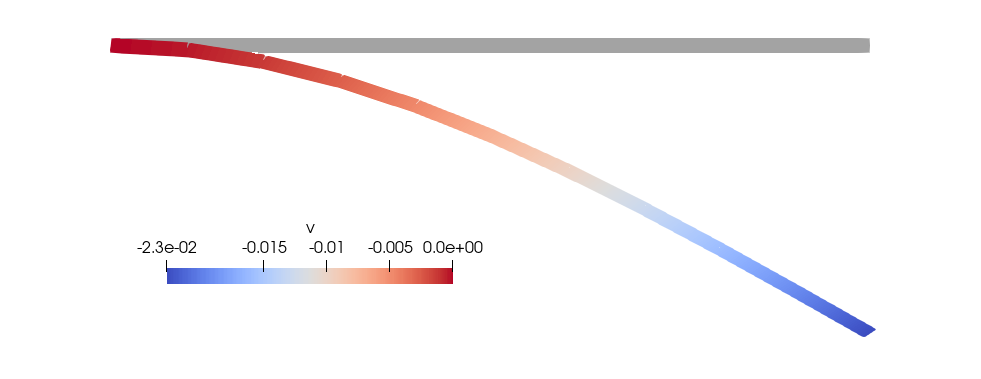
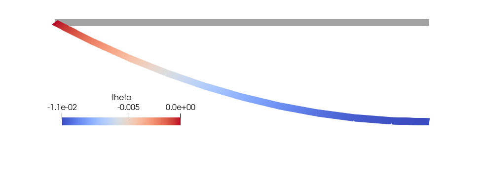
One thing to highlight in the previous figures is that, in contrast with the Euler-Bernoulli beam, the rotations are continuos. That is because the rotations belong to a continuous Finite Element space by construction.

We can also compare the solution to the exact analytical value. In that case we evaluate the value at the tip of the beam, which should be given by

$$v_e=\frac{FL^3}{3EI}$$

Executing the following lines will give us the values of the computed solution, exact solution and the error between the two:

xₚ = Point((L,))
vₑ(t) = F*L^3/(3*EI(t))
println("Computed solution: $(vₕ(xₚ)), Exact solution: $(vₑ(t₀)), Error: $(abs(vₕ(xₚ)-vₑ(t₀)))")

Shear Locking

One of the well-known issues in Finite Element formulations of Timoshenko beams is the shear locking phenomena (not discussed in detail in this tutorial). This problem appears when the thickness tends to zero, i.e. slender beams.

To illustrate this issue, let us compute the value of the tip deflection normalized by the exact value ($v_h/v_e$) for a range of $t$s.

ts = Float64[]
v_rel = Float64[]
for i in 0:10
  tᵢ = 2.0^(-float(i))
  vₕ,θₕ = solve(op(tᵢ))
  push!(ts,tᵢ)
  push!(v_rel,abs(vₕ(xₚ)/vₑ(tᵢ)))
end

We can plot these values using the Plots package:

using Plots
plt = plot(xlabel="t",ylabel="vₕ/vₑ",title="Shear Locking",legend=:bottomright,xscale=:log10,yscale=:log10)
plot!(plt,ts,v_rel,marker=:circle,label="Galerkin")
plot!(plt,ts,ones(length(ts)),ls=:dash,color=:black,label=false)
display(plt)

In the previous plot we clearly see that the deflection of the computed solution relative to the exact solution decreases as we decrease the beam thickness. To addess the issue of shear locking, here we propose three different solution strategies:

1. Sub-integration: use a quadrature rule with lower degree for the terms involving the rotations.

2. Consistent FE spaces: use FE spaces $v_h\in\mathcal{V}_h$ and $\theta_h\in\mathcal{\Theta}_h$ such that $\nabla v_h\in\mathcal{\Theta}_h$.

3. Stabilized formulation: add additional terms to the weak form that prevent shear locking.

Sub-integration

The first approach to solve the shear-locking issue is by using an integration quadrature that only evaluates the function at one quadrature point (at the cell center). This is done by specifying the degree to be integrated exactly with the quadrature rule, which for one quadrature point is 1.

dΩ₁ = Measure(Ω,1)

We now define a different bilinear operator with the split integral, and the corresponding AffineOperator.

a₁(t,(v,θ),(w,ψ)) = ∫( GA(t)*(∇(v)⋅∇(w)) )dΩ + ∫( EI(t)*(∇(θ)⊙∇(ψ)) + GA(t)*((-∇(v)⋅ψ-θ⋅∇(w)+θ⋅ψ)) )dΩ₁
op₁(t) = AffineFEOperator((x,y)->a₁(t,x,y),l,Xₕ,Yₕ)

If we follow the same procedure as before, we can compute and plot the deflection at the beam tip.

v_rel₁ = Float64[]
for tᵢ in ts
  vₕ,θₕ = solve(op₁(tᵢ))
  push!(v_rel₁,abs(vₕ(xₚ)/vₑ(tᵢ)))
end

plot!(plt,ts,v_rel₁,marker=:square,label="Sub-integration")
display(plt)

We see in the plot that the solution with sub-integration now has a relative deflection $v_h/v_e\approx 1.0$.

Consistent FE spaces

The second approach is to define the Finite Element spaces in a way that they satisfy certain stability conditions. In particular, we will use the so called Q2/Q1 element, where the deflection is defined with a 2nd order Lagrange polynomial reference Finite Element and the rotations as a 1st order Lagrange polynomial. Note that in that case, when we take the derivative of the deflection ($\nabla v_h$) it will have the same order as the rotations ($\theta_h$). This approach is also denoted as Consistent Interpolation Elements as proposed by Reddy^[1].

[1]	Reddy, J. (1997). On locking-free shear deformable beam finite elements. Computer Methods in Applied Mechanics and Engineering, 149(1-4), 113-132.

In this case, we don't change the weak form of the problem, but we use different orders for the deflection and rotation reference elements.

order = 2
reffeᵥ₂ = ReferenceFE(lagrangian,Float64,order)
reffeθ₂ = ReferenceFE(lagrangian,VectorValue{1,Float64},order-1)
Vₕ₂ = TestFESpace(Ω,reffeᵥ₂,dirichlet_tags="left")
Ψₕ₂ = TestFESpace(Ω,reffeθ₂,dirichlet_tags="left")
Uₕ₂ = TrialFESpace(Vₕ₂,0.0)
Θₕ₂ = TrialFESpace(Ψₕ₂,VectorValue(0.0))
Xₕ₂ = MultiFieldFESpace([Uₕ₂,Θₕ₂])
Yₕ₂ = MultiFieldFESpace([Vₕ₂,Ψₕ₂])
op₂(t) = AffineFEOperator((x,y)->a(t,x,y),l,Xₕ₂,Yₕ₂)

If we compute the solution for a range of thicknes and plot the relative beam deflection at the tip, we see that this approach also addresses the shear locking phenomena.

v_rel₂ = Float64[]
for tᵢ in ts
  vₕ,θₕ = solve(op₂(tᵢ))
  push!(v_rel₂,abs(vₕ(xₚ)/vₑ(tᵢ)))
end

plot!(plt,ts,v_rel₂,marker=:diamond,label="Q2/Q1")
display(plt)

Stabilized formulation

The last approach is to use a stabilized formulation. That is, to add additional terms into the weak form that are still consistent with the solution, but introduce additional stability properties to the final discrete form. We refer the reader to the work of Aguirre et al^[2] for a comprehensive description of this approach and possible variations.

[2]	Aguirre, A., Codina, R., & Baiges, J. (2023). A variational multiscale stabilized finite element formulation for Reissner–Mindlin plates and Timoshenko beams. Finite Elements in Analysis and Design, 217, 103908.

In this case, the final discrete form is:

$$\int_\Omega \left[\left(EI-\tau_v GA^2\right) \nabla\theta_h:\nabla\psi_h + \ GA\left(1-\tau_\theta GA\right)\left(\nabla v-\theta\right)\left(\nabla w-\psi\right)\right]dΩ = \int_{\Gamma_r} V_N w_h\ d\Gamma$$

where $\tau_v=(c₃GA/h^2+c₄(GA^2/EI))^{-1}$ and $\tau_\theta = (c₁EI/h^2+c₂GA)^{-1}$. With $c₁ = 12.0$, $c₂ = 1.0$, $c₃ = 12.0$, $c₄ = 1.0$ and $h$ the element length.

h = L/partition[1]
c₁ = 12.0; c₂ = 1.0; c₃ = 12.0; c₄ = 1.0
τᵥ(t) = 1.0/(c₃*GA(t)/(h^2)+c₄*(GA(t)^2/EI(t)))
τθ(t) = 1.0/(c₁*EI(t)/(h^2)+c₂*GA(t))
a₃(t,(v,θ),(w,ψ)) = ∫( (EI(t)-τᵥ(t)*GA(t)^2)*(∇(θ)⊙∇(ψ)) + GA(t)*(1-τθ(t)*GA(t))*((∇(v)-θ)⋅(∇(w)-ψ)) )dΩ
op₃(t) = AffineFEOperator((x,y)->a₃(t,x,y),l,Xₕ,Yₕ)

v_rel₃ = Float64[]
for tᵢ in ts
  vₕ,θₕ = solve(op₃(tᵢ))
  push!(v_rel₃,abs(vₕ(xₚ)/vₑ(tᵢ)))
end

plot!(plt,ts,v_rel₃,marker=:utriangle,label="Stabilized")
display(plt)

If we plot the relative values of solution at the tip with respect the exact solution, we also see that the locking phenomena is not present with this approach.

Full script

module Timoshenko
using Gridap

# Discrete model
L = 3.0
domain = (0,L)
partition = (10,)
model = CartesianDiscreteModel(domain,partition)

# Boundary labels
labels = get_face_labeling(model)
add_tag_from_tags!(labels,"left",[1])
add_tag_from_tags!(labels,"right",[2])

# Triangulations
Ω = Triangulation(model)
Γₗ = Boundary(Ω,tags="left")
Γᵣ = Boundary(Ω,tags="right")

# FE spaces
order = 1
reffeᵥ = ReferenceFE(lagrangian,Float64,order)
reffeθ = ReferenceFE(lagrangian,VectorValue{1,Float64},order)
Vₕ = TestFESpace(Ω,reffeᵥ,dirichlet_tags="left")
Ψₕ = TestFESpace(Ω,reffeθ,dirichlet_tags="left")
Uₕ = TrialFESpace(Vₕ,0.0)
Θₕ = TrialFESpace(Ψₕ,VectorValue(0.0))
Xₕ = MultiFieldFESpace([Uₕ,Θₕ])
Yₕ = MultiFieldFESpace([Vₕ,Ψₕ])

# Integration measures and normals
dΩ = Measure(Ω,2*order)
dΓᵣ = Measure(Γᵣ,2*order)

# Problem parameters
b =1.0
E = 1.0e6
ν = 0.2
G = E/(2*(1+ν))
EI(t) = b/12*t^3*E
GA(t) = G*t*b
F = -1.0

# Weak form
a(t,(v,θ),(w,ψ)) = ∫( EI(t)*(∇(θ)⊙∇(ψ)) + GA(t)*((∇(v)-θ)⋅(∇(w)-ψ)) )dΩ
l((w,ψ)) = ∫( F*w )dΓᵣ
op(t) = AffineFEOperator((x,y)->a(t,x,y),l,Xₕ,Yₕ)

# Solution
t₀ = 0.1
vₕ,θₕ = solve(op(t₀))

# Postprocessing
writevtk(Ω,"Timoshenko_solution",cellfields=["v"=>vₕ,"theta"=>θₕ])
xₚ = Point((L,))
vₑ(t) = F*L^3/(3*EI(t))
println("Computed solution: $(vₕ(xₚ)), Exact solution: $(vₑ(t₀)), Error: $(abs(vₕ(xₚ)-vₑ(t₀)))")

# Shear Locking
ts = Float64[]
v_rel = Float64[]
for i in 0:10
  tᵢ = 2.0^(-float(i))
  vₕ,θₕ = solve(op(tᵢ))
  push!(ts,tᵢ)
  push!(v_rel,abs(vₕ(xₚ)/vₑ(tᵢ)))
end

# Plot results
using Plots
plt = plot(xlabel="t",ylabel="vₕ/vₑ",title="Shear Locking",legend=:bottomright,xscale=:log10,yscale=:log10)
plot!(plt,ts,v_rel,marker=:circle,label="Galerkin")
plot!(plt,ts,ones(length(ts)),ls=:dash,color=:black,label=false)
display(plt)

# Solution 1: subintegration
dΩ₁ = Measure(Ω,1)
a₁(t,(v,θ),(w,ψ)) = ∫( GA(t)*(∇(v)⋅∇(w)) )dΩ + ∫( EI(t)*(∇(θ)⊙∇(ψ)) + GA(t)*((-∇(v)⋅ψ-θ⋅∇(w)+θ⋅ψ)) )dΩ₁
op₁(t) = AffineFEOperator((x,y)->a₁(t,x,y),l,Xₕ,Yₕ)
v_rel₁ = Float64[]
for tᵢ in ts
  vₕ,θₕ = solve(op₁(tᵢ))
  push!(v_rel₁,abs(vₕ(xₚ)/vₑ(tᵢ)))
end

# Plot results with subintegration
plot!(plt,ts,v_rel₁,marker=:square,label="Sub-integration")
display(plt)

# Solution 2: compatible spaces
order = 2
reffeᵥ₂ = ReferenceFE(lagrangian,Float64,order)
reffeθ₂ = ReferenceFE(lagrangian,VectorValue{1,Float64},order-1)
Vₕ₂ = TestFESpace(Ω,reffeᵥ₂,dirichlet_tags="left")
Ψₕ₂ = TestFESpace(Ω,reffeθ₂,dirichlet_tags="left")
Uₕ₂ = TrialFESpace(Vₕ₂,0.0)
Θₕ₂ = TrialFESpace(Ψₕ₂,VectorValue(0.0))
Xₕ₂ = MultiFieldFESpace([Uₕ₂,Θₕ₂])
Yₕ₂ = MultiFieldFESpace([Vₕ₂,Ψₕ₂])
op₂(t) = AffineFEOperator((x,y)->a(t,x,y),l,Xₕ₂,Yₕ₂)
v_rel₂ = Float64[]
for tᵢ in ts
  vₕ,θₕ = solve(op₂(tᵢ))
  push!(v_rel₂,abs(vₕ(xₚ)/vₑ(tᵢ)))
end

# Plot results with compatible spaces
plot!(plt,ts,v_rel₂,marker=:diamond,label="Q2/Q1")
display(plt)

# Solution 3: Stabilized formulation
h = L/partition[1]
c₁ = 12.0; c₂ = 1.0; c₃ = 12.0; c₄ = 1.0
τᵥ(t) = 1.0/(c₃*GA(t)/(h^2)+c₄*(GA(t)^2/EI(t)))
τθ(t) = 1.0/(c₁*EI(t)/(h^2)+c₂*GA(t))
a₃(t,(v,θ),(w,ψ)) = ∫( (EI(t)-τᵥ(t)*GA(t)^2)*(∇(θ)⊙∇(ψ)) + GA(t)*(1-τθ(t)*GA(t))*((∇(v)-θ)⋅(∇(w)-ψ)) )dΩ
op₃(t) = AffineFEOperator((x,y)->a₃(t,x,y),l,Xₕ,Yₕ)
v_rel₃ = Float64[]
for tᵢ in ts
  vₕ,θₕ = solve(op₃(tᵢ))
  push!(v_rel₃,abs(vₕ(xₚ)/vₑ(tᵢ)))
end

# Plot results with stabilized formulation
plot!(plt,ts,v_rel₃,marker=:utriangle,label="Stabilized")
display(plt)
end