Strong vs weak boundary conditions

In this tutorial we will learn how to enforce strong and weak Dirichlet boundary conditions in a simple 2D Poisson problem.

In addition, in this tutorial we will also learn the following Gridap features:

Tag different geometrical entities of a CartesianDiscreteModel
Define different boundary triangulations depending on the tags

Problem setting

Here we consider the 2D Poisson problem and associated boundary conditions:

\begin{aligned} -\Delta u&= f\qquad&\text{in $\Omega$},\\ u &= u_1\qquad&\text{in $\Gamma_l\cup\Gamma_r$},\\ u &= u_0\qquad&\text{in $\Gamma_b\cup\Gamma_t$}. \end{aligned}

Where $\Gamma_l$ , $\Gamma_r$ , $\Gamma_b$ and $\Gamma_t$ are the left, right, bottom and top boundaries, respectively. In all these boundaries we enforce Dirichlet boundary condition with prescribed value of $u_1(x,y)=y*(L-y)$ and $u_0(x,y)=0.0$ , where $L$ is the square side size..

Domain discretization

Here we will follow the steps definied in tutorial 1, feel free to check this tutorial for in-depth description of all the steps. The main difference is that here we use a two-dimensional domain defined by a square of size $L=3.0$ , discretized using 10 elements per direction.

using Gridap

L = 3.0
domain = (0.0, L, 0.0, L)
partition = (10, 10)
model = CartesianDiscreteModel(domain, partition)

We tag the left, right, bottom and top boundaries to apply boundary conditions later on, and we define interior and boundary triangulations:

labels = get_face_labeling(model)
add_tag_from_tags!(labels, "left", [1,3,7])
add_tag_from_tags!(labels, "right", [2,4,8])
add_tag_from_tags!(labels, "bottom", [5])
add_tag_from_tags!(labels, "top", [6])

Ω = Interior(model)
Γl = Boundary(model, tags="left")
Γr = Boundary(model, tags="right")
Γb = Boundary(model, tags="bottom")
Γt = Boundary(model, tags="top")

In a 2D setting, the default entities are numbered in ascending order from lower topological dimension to higher topological dimension and following a left-right and bottom-top ordering within each dimension. To clarigy concepts, in a 2D cartesian model we will have the following geometrical entities:

Vertices (topological dimension $0$ ):
- Bottom-left -> 1
- Bottom-right -> 2
- Top-left -> 3
- Top-right -> 4
Edges (topological dimension $1$ ):
- Aligned with x-axis at the bottom -> 5
- Aligned with x-axis at the top -> 6
- Aligned with y-axis at the left -> 7
- Aligned with y-axis at the right -> 8
Surfaces (topological dimension $2$ ):
- Interior domain -> 9

3---6---4
|       |
7   9   8
|       |
1---5---2

Finite Element spaces

In this tutorial we will use lagrangian reference Finite Elements of arbitrary order order, which we will set to 1 initially. We then construct the test and trial Finite Element spaces for the test function and the unknown, respectively. Here we will first consider the case of strongly enforcement of the Dirichlet boundary conditions. In that case, we specify a vector of tags in the TestFESPace and a vector with the Dirichlet boundary condition value in the TrialFESpace, one value per tag.

order = 1
reffe = ReferenceFE(lagrangian, Float64, order)
Vₕ₀ = TestFESpace(model, reffe,dirichlet_tags=["left","right","bottom","top"])
Uₕᵤ = TrialFESpace(Vₕ₀,[u₁,u₁,u₀,u₀])

Discrete form.

Without going into the details of the derivation, the final discrete form of the problem reads: find $u_h\in\mathcal{V}_h^u$ such that

\int_\Omega \nabla u_h\cdot\nabla v_h d\Omega = \int_{\Omega} fv_h\ d\Omega\qquad \forall v_h\in\mathcal{V}_h^0

Again, before implementing the discrete form, we define the integration measures and problem parameters.

degree = 2*order
dΩ = Measure(Ω, degree)

f(x) = 1.0

With all the ingredients in place we can now define the discrete form, where we will use the AffineFEOperator taking advantage of the fact that the formulation is linear.

a(u,v) = ∫(∇(v)⋅∇(u))dΩ
b(v) = ∫(f*v)dΩ
op₀ = AffineFEOperator(a,b,Uₕᵤ,Vₕ₀)

Weak imposition of boundary conditions

To enforce the Dirichlet boundary conditions in a weak sense, we start by defining the Finite Element spaces without any constrain in the boundary.

Vₕ = TestFESpace(model, reffe)
Uₕ = TrialFESpace(Vₕ)

Then the Dirichlet boundary condition will be enforced through the weak form instead of restricting the space of FE functions. Here we use the Nitsche's method ^[1].

^[1] [1] J. Nitsche, Über ein Variationsprinzip zur Lösung von Dirichlet-Problemen bei Verwendung von Teilräumen, die keinen Randbedingungen unterworfen sind, Abhandlungen aus dem mathematischen Seminar der Universität Hamburg, Springer, 1971. (In German)

The main idea of this approach is to keep the terms that come from the integration by parts of the laplacian and add two additional terms that are consistent with the boundary condition. First, a term that is symmetric (or skewsymmetric) with respect to the integration by parts term. Second, a penalty term that penalizes the difference between the solution and the boundary condition value at the Dirichlet boundaries. The final weak form for this case reads: find $u_h\in\mathcal{V}_h$ such that

\begin{aligned} &\int_\Omega \nabla u_h\cdot\nabla v_h d\Omega\, + \int_{\partial\Omega}\left( \frac{\alpha}{h} v_h(u_h-u_D)- (\mathbf{n}\cdot\nabla u_h)v_h - (\mathbf{n}\cdot\nabla v_h)(u_h-u_D) \right)dΓ \\ &= \int_{\Omega} fv_h\ d\Omega\qquad \forall v_h\in\mathcal{V}_h \end{aligned}

Where $\alpha$ is a penalty parameter that can be tuned to five more weight to the penalty term. In this tutorial we select $\alpha=10.0$ . If we split the boundary integrals for each boundary of our domain, we have:

\begin{aligned} &\int_\Omega \nabla u_h\cdot\nabla v_h d\Omega\ +\\ &\int_{\Gamma_l}\left( \frac{\alpha}{h} v_h(u_h-u_1) - (\mathbf{n}_l\cdot\nabla u_h)v_h - (\mathbf{n}_l\cdot\nabla v_h)(u_h-u_1) \right) dΓ +\\ &\int_{\Gamma_r}\left( \frac{\alpha}{h} v_h(u_h-u_1) -(\mathbf{n}_r\cdot\nabla u_h)v_h - (\mathbf{n}_r\cdot\nabla v_h)(u_h-u_1) \right)dΓ +\\ &\int_{\Gamma_b}\left( \frac{\alpha}{h} v_h(u_h-u_0) -(\mathbf{n}_b\cdot\nabla u_h)v_h - (\mathbf{n}_b\cdot\nabla v_h)(u_h-u_0) \right) dΓ\\ &\int_{\Gamma_t}\left( \frac{\alpha}{h} v_h(u_h-u_0) -(\mathbf{n}_t\cdot\nabla u_h)v_h - (\mathbf{n}_t\cdot\nabla v_h)(u_h-u_0) \right) dΓ \\ &= \int_{\Omega} fv_h\ d\Omega\qquad \forall v_h\in\mathcal{V}_h \end{aligned}

As you can see, in the previous weak form we need the definition of the integration measures at the different boundaries and the normal vector to these boundaries.

dΓl = Measure(Γl, degree)
dΓr = Measure(Γr, degree)
dΓb = Measure(Γb, degree)
dΓt = Measure(Γt, degree)
nl = get_normal_vector(Γl)
nr = get_normal_vector(Γr)
nb = get_normal_vector(Γb)
nt = get_normal_vector(Γt)

With the normals and measures, we can now define the final weak form and affine FE operator for the Nitsche approach:

h = L/partition[1]
γ = 10.0/h
a₁(u,v) = ∫(∇(v)⋅∇(u))dΩ +
          ∫( γ*(v*u) - (nl⋅∇(u))*v - (nl⋅∇(v))*u)dΓl +
          ∫( γ*(v*u) - (nr⋅∇(u))*v - (nr⋅∇(v))*u)dΓr +
          ∫( γ*(v*u) - (nb⋅∇(u))*v - (nb⋅∇(v))*u)dΓb +
          ∫( γ*(v*u) - (nt⋅∇(u))*v - (nt⋅∇(v))*u)dΓt
b₁(v) = ∫(f*v)dΩ +
        ∫( γ*(v*u₁) - (nl⋅∇(v))*u₁)dΓl +
        ∫( γ*(v*u₁) - (nr⋅∇(v))*u₁)dΓr +
        ∫( γ*(v*u₀) - (nb⋅∇(v))*u₀)dΓb +
        ∫( γ*(v*u₀) - (nt⋅∇(v))*u₀)dΓt
op₁ = AffineFEOperator(a₁,b₁,Uₕ,Vₕ)

Solution and postprocessing

With the different Finite Operator defined, we can solve the problem for the two cases, strong and weak Dirichlet boundary conditions enforcement.

uₕ₀ = solve(op₀)
uₕ₁ = solve(op₁)

As usual, we can postrpocess the solution using Paraview:

writevtk(Ω,"solution",cellfields=["u_strong"=>uₕ₀,"u_weak"=>uₕ₁])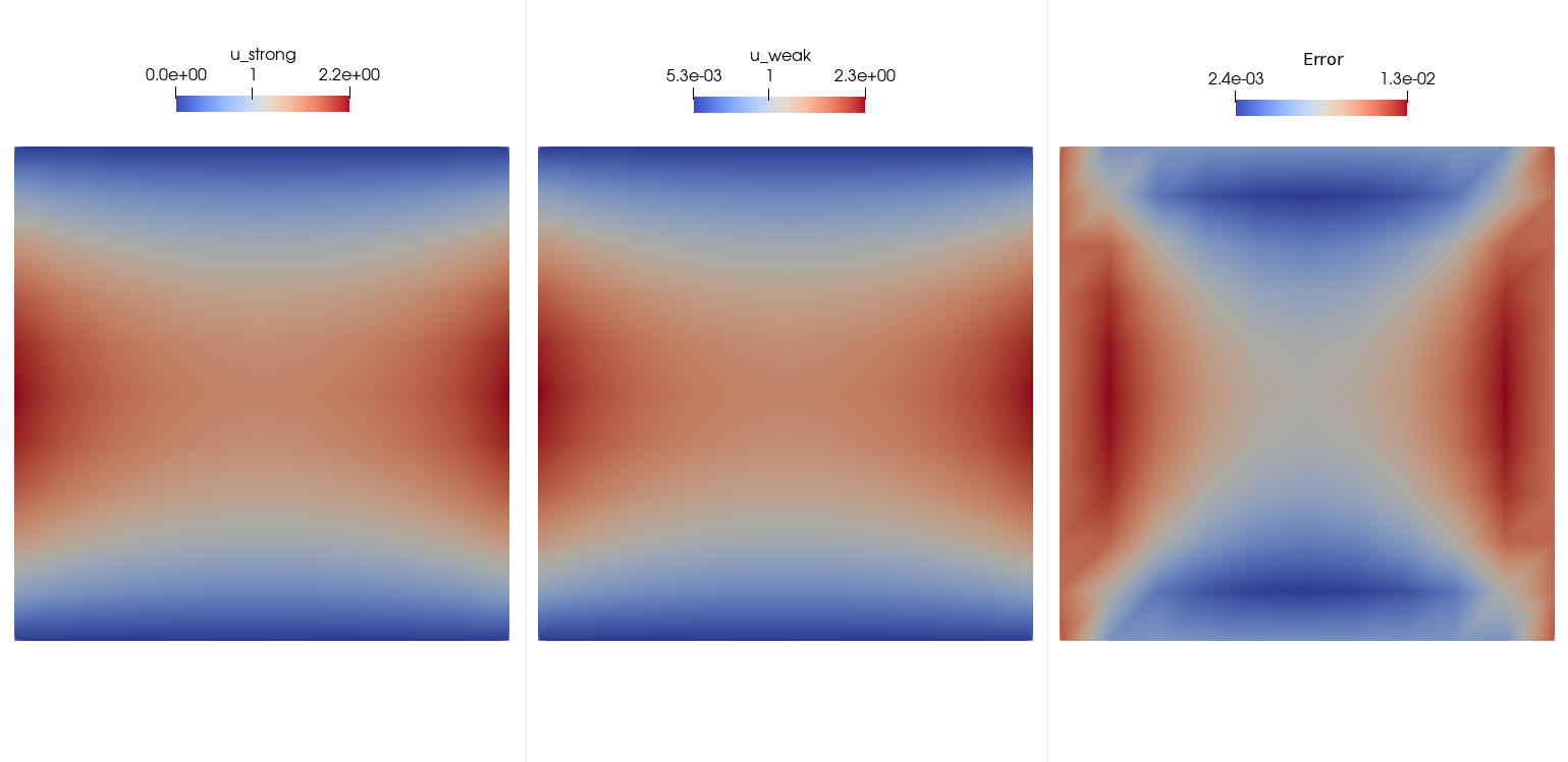

Solution for the strong Dirichlet BCs (left), weak Dirichlet BCs (center) and error between the two (right)

We can also compute the norm of the difference between the two solutions by executing the following line

println(√(∑(∫((uₕ₀-uₕ₁)*(uₕ₀-uₕ₁))dΩ)))

Full script

module Poisson_weakBCs
using Gridap

# Define the model
L = 3.0
domain = (0.0, L, 0.0, L)
partition = (10, 10)
model = CartesianDiscreteModel(domain, partition)

# Define boundaries
labels = get_face_labeling(model)
add_tag_from_tags!(labels, "left", [1,3,7])
add_tag_from_tags!(labels, "right", [2,4,8])
add_tag_from_tags!(labels, "bottom", [5])
add_tag_from_tags!(labels, "top", [6])

# Triangulations
Ω = Interior(model)
Γl = Boundary(model, tags="left")
Γr = Boundary(model, tags="right")
Γb = Boundary(model, tags="bottom")
Γt = Boundary(model, tags="top")

# Boundary conditions
u₀(x) = 0.0
u₁(x) = x[2]*(L-x[2])

# FE spaces
order = 1
reffe = ReferenceFE(lagrangian, Float64, order)
Vₕ₀ = TestFESpace(model, reffe,dirichlet_tags=["left","right","bottom","top"])
Uₕᵤ = TrialFESpace(Vₕ₀,[u₁,u₁,u₀,u₀])

# Measures
degree = 2*order
dΩ = Measure(Ω, degree)

# Weak formulation strong Dirichlet
f(x) = 1.0
a(u,v) = ∫(∇(v)⋅∇(u))dΩ
b(v) = ∫(f*v)dΩ
op₀ = AffineFEOperator(a,b,Uₕᵤ,Vₕ₀)

# solve
uₕ₀ = solve(op₀)

# FE spaces with no strong Dirichlet
Vₕ = TestFESpace(model, reffe)
Uₕ = TrialFESpace(Vₕ)

# Additional measures on boundaries
dΓl = Measure(Γl, degree)
dΓr = Measure(Γr, degree)
dΓb = Measure(Γb, degree)
dΓt = Measure(Γt, degree)

# Normal vectors
nl = get_normal_vector(Γl)
nr = get_normal_vector(Γr)
nb = get_normal_vector(Γb)
nt = get_normal_vector(Γt)

# Weak formulation weak Dirichlet
h = L/partition[1]
γ = 10.0/h
a₁(u,v) = ∫(∇(v)⋅∇(u))dΩ +
          ∫( γ*(v*u) - (nl⋅∇(u))*v - (nl⋅∇(v))*u)dΓl +
          ∫( γ*(v*u) - (nr⋅∇(u))*v - (nr⋅∇(v))*u)dΓr +
          ∫( γ*(v*u) - (nb⋅∇(u))*v - (nb⋅∇(v))*u)dΓb +
          ∫( γ*(v*u) - (nt⋅∇(u))*v - (nt⋅∇(v))*u)dΓt
b₁(v) = ∫(f*v)dΩ +
        ∫( γ*(v*u₁) - (nl⋅∇(v))*u₁)dΓl +
        ∫( γ*(v*u₁) - (nr⋅∇(v))*u₁)dΓr +
        ∫( γ*(v*u₀) - (nb⋅∇(v))*u₀)dΓb +
        ∫( γ*(v*u₀) - (nt⋅∇(v))*u₀)dΓt
op₁ = AffineFEOperator(a₁,b₁,Uₕ,Vₕ)

# solve
uₕ₁ = solve(op₁)

# Output solution to vtk
writevtk(Ω,"solution",cellfields=["u_strong"=>uₕ₀, "u_weak"=>uₕ₁])

# Print error
println(√(∑(∫((uₕ₀-uₕ₁)*(uₕ₀-uₕ₁))dΩ)))

end